I Fed Sam Vecenie's Draft Guides Into Python

TF-IDF vectors, UMAP scatterplots, and player neighborhoods

I enjoy

Sam Vecenie

’s work. His yearly draft guides are a must-read for me. They are detailed and easy to follow, and they give a draft casual like me enough information to feel fully informed and ready to armchair GM all summer. There is a lot of good material in those guides.

There is, of course, valuable signal in Sam’s description of the prospects. But I’ve also wondered whether there might be some interesting signal in how Sam describes certain prospects. Are there patterns in the ways Sam evaluates players? And, if so, do those patterns stay consistent across different draft classes? Basically, I wanted to see if I could reverse-engineer a set of Vecenie player comparisons directly from the text itself.

Here’s how it turned out:

---

Parsing the Draft Guides

I started by extracting the text from the draft guides, year by year. I converted each PDF to text, then wrote a script that parsed the text into different categories for each player (which are already helpfully cleanly laid out in the draft guides): background section, strengths, weaknesses, and summary. Once I was able to pull all of these categories for each player, I combined them all into one dataset containing a collection of Sam’s writeups from 2020 to 2025.

---

TF-IDF and Cosine Similarity

At this point, I should admit that I am a beginner in this area. I have been listening to a machine learning podcast/audiobook that walks through some basic natural language processing ideas, and that gave me enough confidence to try something simple. I wanted a first step that was easy to implement, easy to interpret, and widely used in introductory text analysis. That led me to TF-IDF and cosine similarity.

If you are not familiar with these, TF-IDF (term frequency–inverse document frequency) is a way of turning text into numbers. The term frequency part counts how often a word appears in a document. The inverse document frequency part reduces the importance of words that show up everywhere, such as “player,” “game,” or “season.” The combined result is a weighted vocabulary that highlights words that matter more to a specific document than to the overall corpus.

TF-IDF aims to answer the question: What are the words that make this player’s writeup distinctive compared to everyone else’s?

Once you have these weighted word vectors for every player, you can compare them. That is where cosine similarity comes in. It measures how close two text vectors are by looking at the angle between them rather than the raw difference in counts. Two writeups that emphasize the same ideas and vocabulary will have a small angle between their vectors and therefore a high similarity score.

I think this method is common for beginners because the logic is simple and the results usually make sense. You do not need anything fancy. You take the text, convert it into numerical vectors using TF-IDF, and then compare the angles between them. I used the standard scikit-learn implementation, which handles all the confusing math for you.

So I built a TF-IDF matrix for all the writeups and computed cosine similarity across every pair of players. This gave me a first look at which prospects Sam described in similar terms. The results made intuitive sense, but the first major issue surfaced immediately. A number of profiles have helpful background information, such as family history, early childhood anecdotes, or a blurb about where the player played in the past. So, these background-heavy entries clustered together even when Vecenie’s analysis of the players themselves had nothing in common on the court. I decided to remove the background information blurbs from the dataset. Once I removed the bio from my dataset, all that remained were the strengths, weaknesses, and summary.

---

UMAP

Once I had cleaned TF-IDF vectors for every player, I wanted a way to see the big-picture structure of the language at a glance. TF-IDF produces high-dimensional data. Each unique word or phrase becomes a separate dimension, which means each player writeup is represented as a point in a space with tens of thousands of dimensions. This stuff breaks my brain.

This led me to UMAP (Uniform Manifold Approximation and Projection), which is a technique used in machine learning to take extremely high-dimensional data and compress it into a lower-dimensional space while trying to preserve the important structure. The main idea behind UMAP is that data often has a natural shape or geometry even when the raw representation looks noisy and huge. UMAP tries to uncover that shape.

I used UMAP to shrink the TF-IDF space to five dimensions. This gave me a more compact version of the language structure that still held onto the meaningful similarities. After that, I projected it into two dimensions so I could visualize it on a scatter plot.

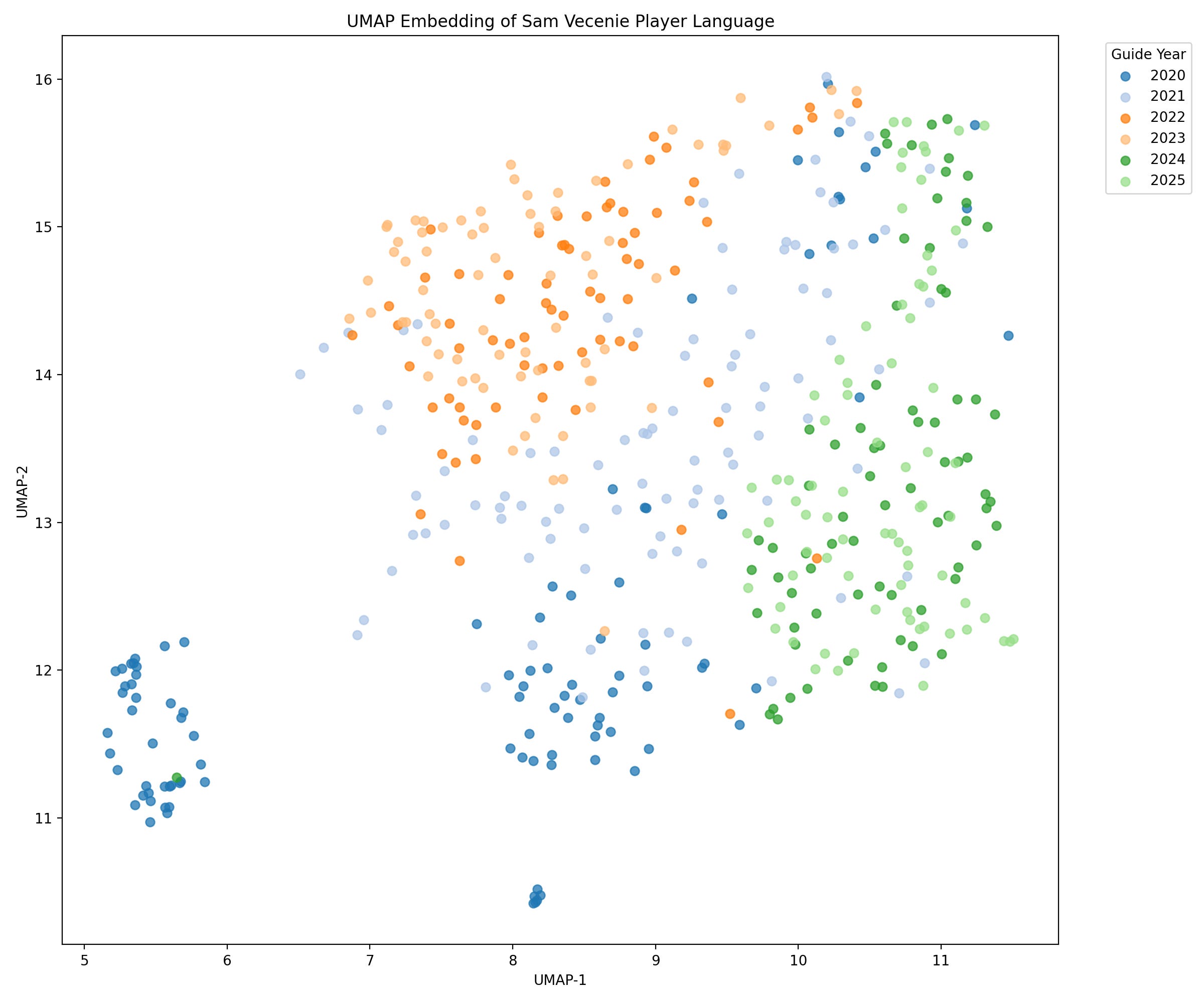
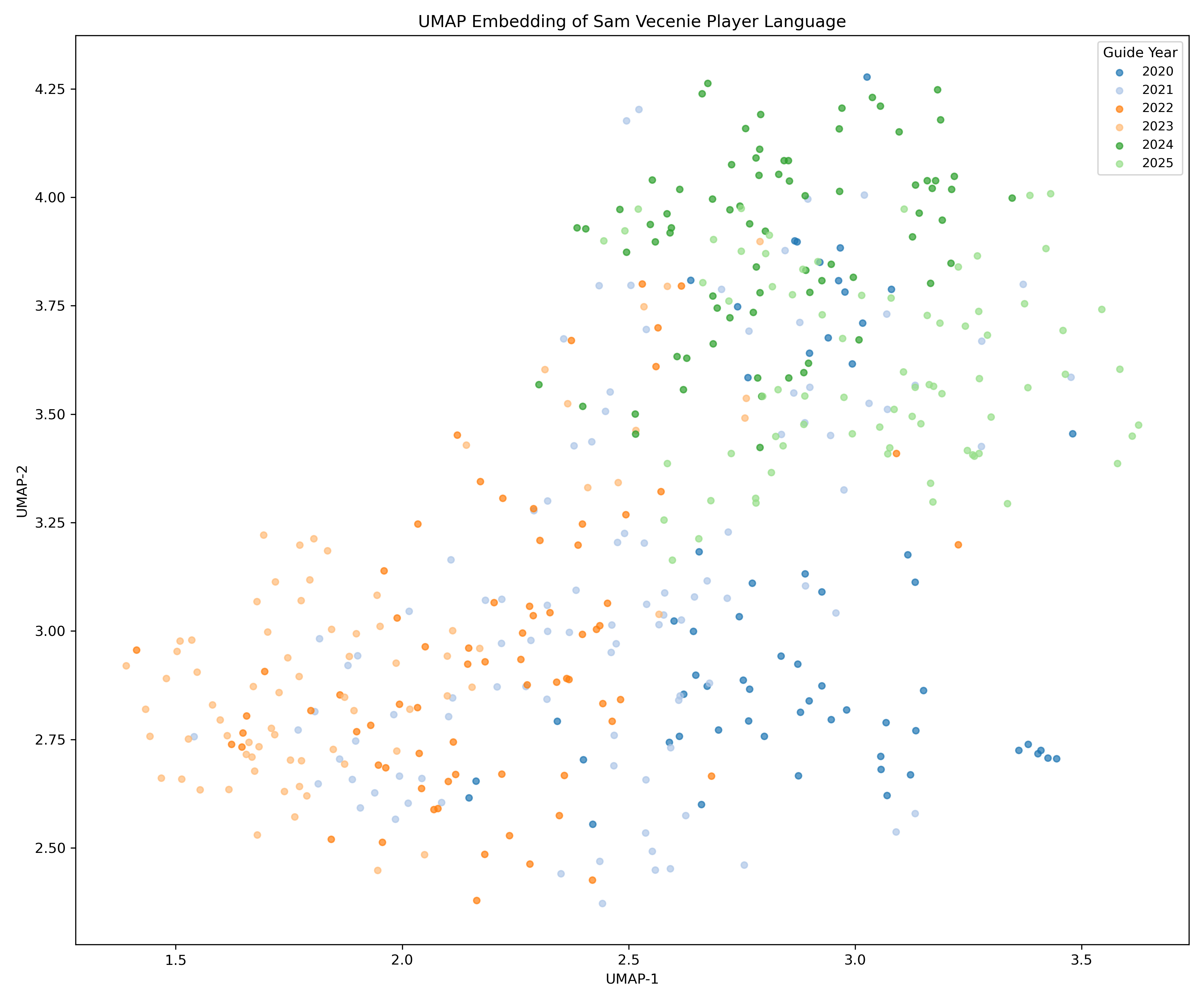
My first thought from this plot is that the bottom left cluster was intriguing. It turns out, this is just a grouping of super short summaries of Sam’s lower-ranked prospects. These writeups are short blurbs and nowhere near as in-depth as the higher-ranked prospects. So, I removed those (and all of the outlier short blurbs throughout). That process left us with this more focused plot:

---

Creating Clusters

Once the UMAP space was ready, the next question was how to group players who sit near one another. To create clusters, I used scikit-learn for K-Means clustering. Essentially, you pick a number of clusters (K) and the algorithm places K points in the space as “centers.” Each player is assigned to the nearest center based on distance. The algorithm then shifts the centers toward the middle of their assigned points and repeats this process until everything stabilizes. When it finishes, each player belongs to a cluster defined by proximity in the UMAP space.

Once the clusters were defined, I wanted to understand why certain players grouped together. To do this, I took the TF-IDF vectors for each cluster and looked for the words that were most distinctive to that group. These are the words that appear often inside the cluster but much less often elsewhere relatively. They give a sense of the themes that tie the writeups together.

Below is a simple sample of the output the TF-IDF analysis produced. These are not interpretations or labels. They are just the words that the model identified as most characteristic of each cluster:

• Cluster 0

  • rim, foot, length, right, bit

• Cluster 1

  • big, center, drop, roll, play

• Cluster 2

  • year, wing, offense, offensive, season

• Cluster 3

  • high level, guard, hit, make, think

• Cluster 4

  • past season, past, bit, foot, gets

• Cluster 5

  • right, way, shots, works, bit

• Cluster 6

  • screens, pull, guard, defenders, point

Here are these clusters visualized:

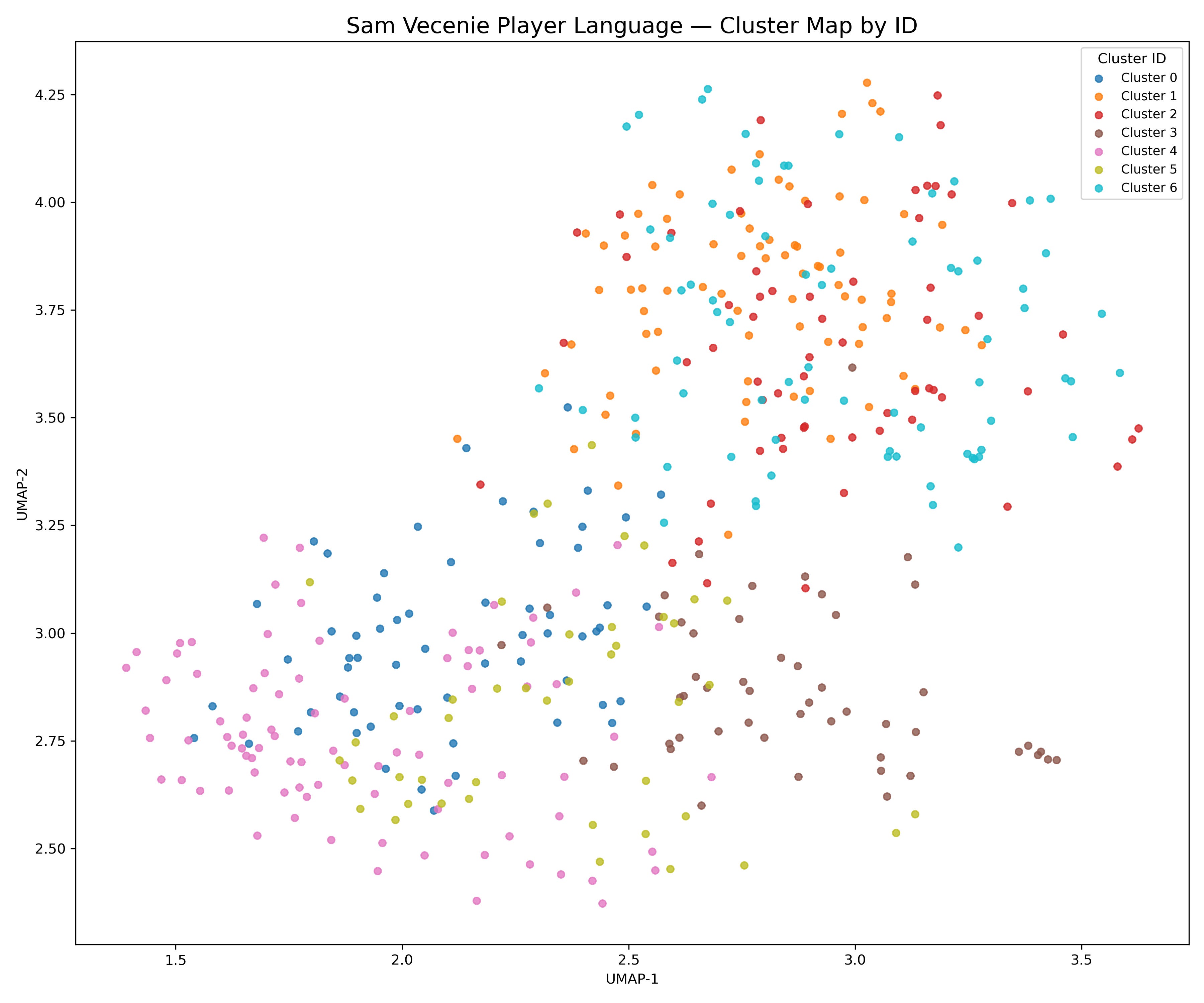
A simple enough next step would be to assign some cluster titles to these groups. I tried, but ultimately struggled too much trying to assign an overarching label. I feel for the draft evaluators who are tasked to do stuff like this. For now, I’ll just leave them as numbered clusters.

---

Specific Player Comparisons

Once the clusters were created and I had a sense of how the language grouped itself, the next question was how to explore the space in a more concrete way. Clusters are helpful, but they are still a bird’s-eye view. I wanted to know what the relationships looked like at the individual player level.

Similarity Scores

Using the TF-IDF vectors and cosine similarity, I can find the players whose scouting writeups share the most language in common. To give a sense of what this looks like, here is an example with Tyrese Maxey:

[info] Target: Tyrese Maxey (2020)

Top neighbors:
- Tyrese Haliburton (2020), cluster_id=0, sim=0.183
- Jalen Hood-Schifino (2023), cluster_id=7, sim=0.176
- Adam Flagler (2023), cluster_id=0, sim=0.174
- Tyrell Terry (2020), cluster_id=0, sim=0.168
- Tre Jones (2020), cluster_id=0, sim=0.162

The higher the score, the more overlap in Sam’s phrasing, emphasis, and wording when describing those players. I ran this for all of the players in the dataset. Here’s a big ol’ table of the data:

To be honest, I’m not really sure how much signal there is in here. I see some and think “oh yeah, those guys are totally comparable,” and I see others and think “oh yeah, I totally messed this up.”

Neighborhoods

For some reason, this whole exercise made me think of players living in neighborhoods with the other players most similar to them. I’m not sure that resonates with anyone else. But it makes sense in my brain.

And so, I created some silly little Python art neighborhoods for each player to visualize their closest neighbors. Again, here’s Tyrese Maxey:

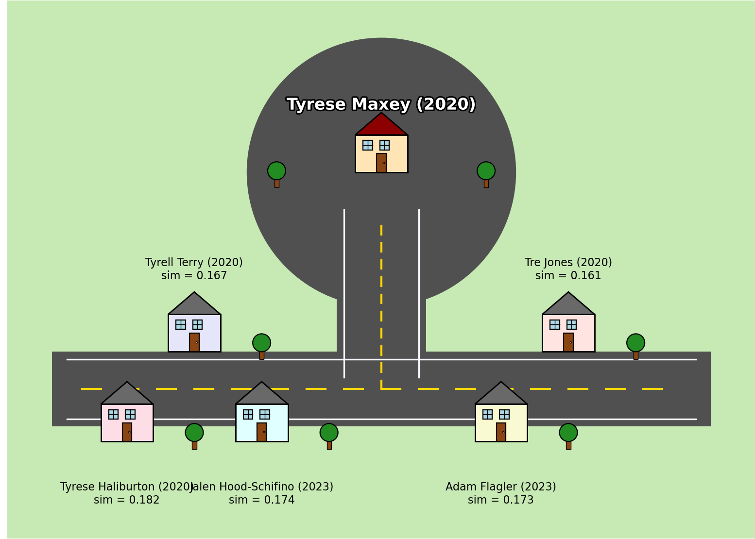
Once I get to the arts and crafts portion of a project, it’s probably a good signal that I should wrap it up pretty soon.

Cross-Year Comparisons

In digging through the similarity scores, I noticed something interesting. The closest neighbors for many players came from the same draft class. At first, this was surprising, but it makes sense. Each year of Sam’s writing likely has its own rhythm and vocabulary (as does anyone’s writing). Certain phrases show up repeatedly within the same guide and not much in others. Certain themes might dominate a particular class.

This is why cross-year comparisons stood out as a plausibly interesting focal point. When a player’s closest matches come from a different draft class, the similarity might reflect something deeper in the language. The model is cutting through the yearly tone and finding cases where Sam used genuinely similar wording to describe two players several years apart.

Here’s a look at the top 1000 cross-year comparisons:

I feel like we get a bit more signal through the noise on these.

These cross-year relationships ended up being one of the more interesting parts of the project. They highlight players who may have very different contexts or roles but whose writeups share the same language. They also help confirm that the model is picking up some patterns in Sam’s evaluative style rather than just the vocabulary of a single draft guide (I think).

---

Future Work

There are a few natural directions this project could go next. One idea is to link this language space to on-court outcomes by merging the similarity scores with early career data such as EPM, efficiency numbers, or role changes. It might also be interesting to extract specific attributes from the text, such as recurring notes about strength, decision making, or shooting mechanics, and see how those attributes cluster on their own. I’ll probably explore these at some point and share if the results are interesting.

It is also worth noting that this project is not meant to be especially serious. I treated it as a learning exercise and a chance to try out a few new skills, not as a rigorous attempt to model scouting theory or extract some deep truth.

I had fun. For now, that’s all I got.